Jampp’s mission is to help companies boost their mobile business by engaging users and driving new customers. Fighting mobile fraud is a top priority to ensure this goal is possible. Other than spamming, phishing and scamming, ad fraud is one of the most profitable scenarios for rogue internet users. With impact forecasts of mobile fraud in 2016 that varied along $1.25bn (Forensiq) and $7.2bn (ANA), we can see how this is a crucial problem in the industry.

Click Spamming

The Invalid Traffic Detection and Filtration Guidelines Addendum made by the Media Rating Council (MRC) and the Mobile Marketing Association (MMA) states that sophisticated fraud is characterized by the need of significant human analysis and intervention to be detected. In our previous fraud post we talked about the different types of fraud in the mobile advertisement industry and in this opportunity we are going to focus on Click Spamming detection.

Click Spamming refers to applications that generate thousands of fake impressions and/or click requests programmatically. The scammer will first run tests to extract appropriate campaign URL tokens for a specific device type or location. Next they will generate thousands of fake impressions and/or clicks which in turn steal the installs’ attribution from other publishers or directly from organic traffic. An advertiser whose campaign is spammed would see huge volumes across clicks and impressions, low CVRs and good in-app-event rates.

To counter this type of fraud we can consider the TimeDelta metric.

TimeDelta

This is the measure of the time it takes between click and install (the first app-open). The idea behind this metric is that, in general, counting data will statistically appear as a distribution which is exponentially decreasing and with long thin tails. In general, empirical distributions that arise from the data can be characterized by these specific properties. Most of the distribution’s mass would be concentrated in smaller Time Delta values, and a small percentage of the distribution would be spread out in higher values.

As an example, we take a look at a group of apps in the Classifieds business. All Time Delta measurements shown are aggregated into the same dataset, where measure is in minutes and data is taken for a day worth of installs. In addition, clicks could have happened anytime previous to the install.

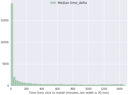
Note that the histogram shows a sharp decay for the lower values of the metric with an almost constant decay value for higher time deltas.

This statistical property in the distributions is ubiquitous across apps of different verticals, countries and platforms. Minor differences can arise between distributions, specifically on the maximum values of the data and in the exact rate of decay. Other than that, there are no notable differences among them, until we take a look at a fraudulent publisher. In our data explorations, we find that we lose the exponential decay of the distribution and we start to see data with fat tails. Two examples from different publishers are shown below:

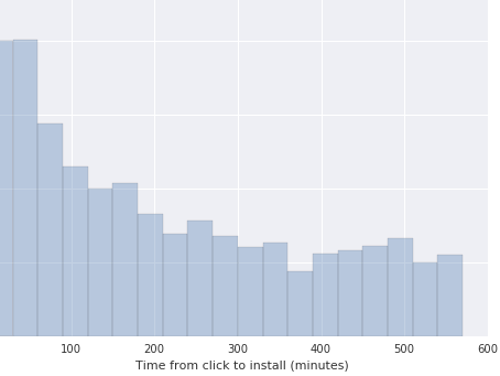
In this image, the decay has become linear and lots of installs are still coming late.

As a last example, we look at a scenario where the distribution is multimodal. At first, the decay and the distribution look like usual, but then the large slump at the end confirms this is a publisher with Click Spamming activity.

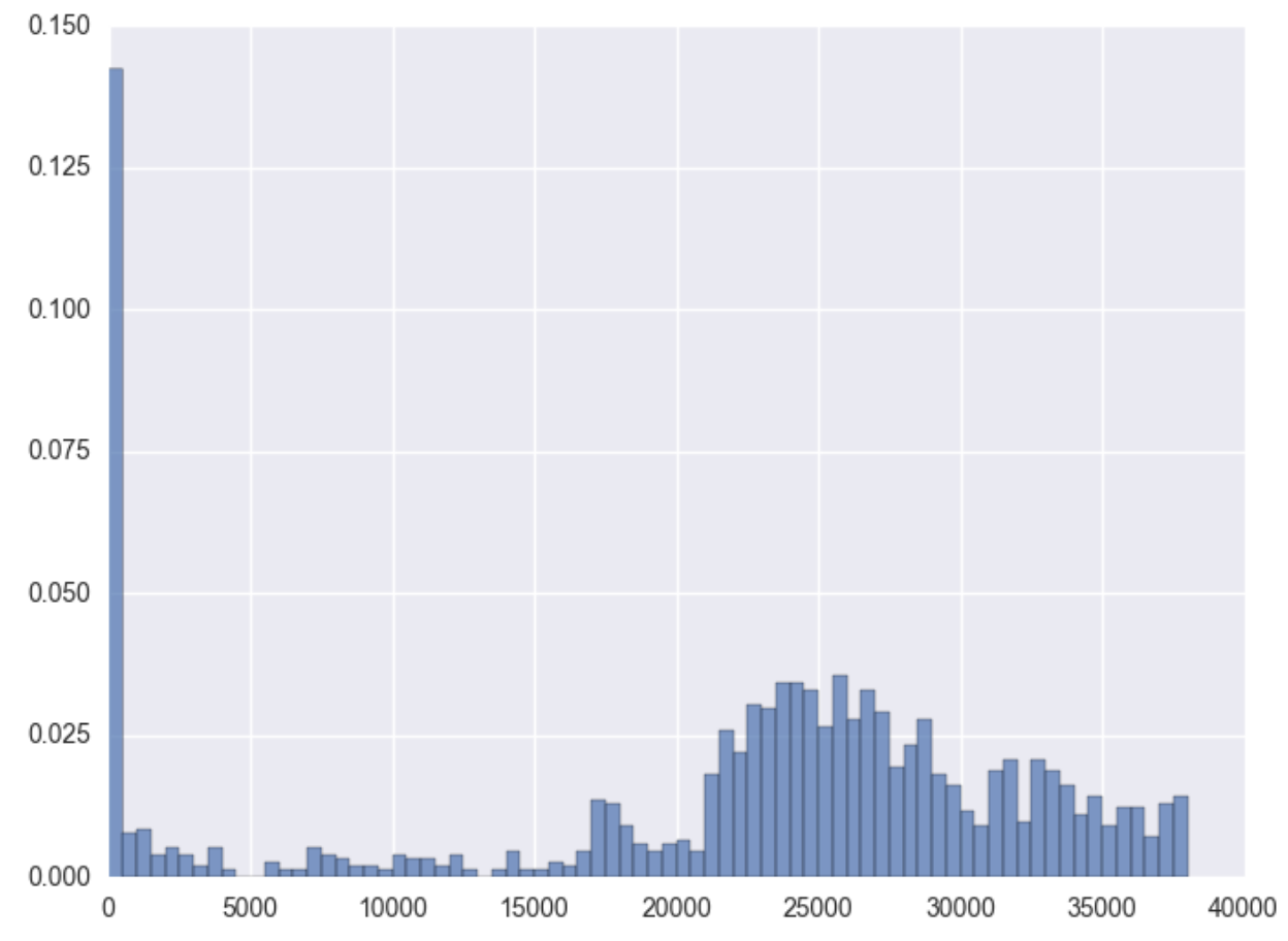
In order to give a response to this fraudulent activity, a detection system needs two things. First, a way of automatically classifying distribution samples as fraudulent or not. Knowing which behavior is clean or fraudulent will help to clean the data and unskew the advertiser’s metrics.

Another desired aspect would be to have a specific threshold from which to draw the line for suspicious installs. Even though there are arguments in favor of the authenticity of in-app opens coming days after the click, we can safely assume that a significant part of late installs come from fraudulent activity. Discarding these wouldn’t have a significant impact on user acquisition business, where in most cases 50% of all global installs arrive in the first hour.

Care must be taken though not to set a universal value for every install from any app, vertical and/or country. Install behavior is varied and a value which fits for regions with fast Internet access and fast smartphones will most probably not fit for a mobile market which is still developing.

Theoretical Aspects

In order to build our system, we must first find a way to identify fraudulent vs. non-fraudulent distributions. As a start, we can make the assumption that all installs’ events are independent or that one event is not related to another. Then we need to choose among distributions which assimilate the exponential decaying nature of TimeDelta. We must also select among functions with infinite support and which only take in positive values.

After various tests and evaluating different candidates, we found out that there are certain distributions that best fit usual TimeDelta behavior: the Exponential ¹, the Exponentiated Weibull ² and the Generalized Extreme Value ³ distributions. Note that the second is an extension of the first one. For more references to the properties of these functions, we recommend following their respective links to Wikipedia.

On the other hand, to identify fraudulent behavior we will try and fit data with two very simple distributions, the Uniform ⁴ and Chi-squared ⁵

They might not be exactly what we’re looking for, but then again, what form does fraudulent activity take and how can we actually build a system that is flexible enough to adapt to changes in the distribution? Here’s the catch: we don’t actually need to accurately model fraudulent distributions. We need these distributions to be slightly better fitting than the usual non-fraudulent distributions. The following paragraph explains this better.

The Kullback-Leibler divergence or relative entropy is a pseudo-metric to assess which of the theoretical samples best fits the empirical sample. This statistic is derived from information theory and has a close resemblance to the entropy of the data (in the information theory sense). It is usually taken as a measure of difference between distributions $Q$ and $P$ where the former is an approximation of the latter. Its definition is

The second form better characterizes how the $Q$ distribution is used as an approximation of $P$ by comparing the entropy $H(P)$, with the entropy when we use $Q$ as an approximation.

For our specific case we will compare the theoretical distribution P with the empirical distribution Q. The idea is to try and decide which category the empirical distribution falls to. And then use the theoretically fit distribution to set the 95th percentile threshold on the data. This ad-hoc percentile will serve as a cut to all late timed installs.

Methodology

On a periodical basis, run the following algorithm to every app’s TimeDelta data:

1. For each theoretical distribution, find the best fitting parameters from the data.
2. Take a theoretical sample which is the same size as the empirical sample, using the aforementioned parameters.
3. Assess, through the KL measure, which is the distribution that fits our data. Make a special record if the distribution has a fraudulent nature.
4. Get the 95th theoretical percentile as our threshold, if the best-fit distribution is non-fraudulent.

Here, we must remind readers that we have chosen weak theoretical distributions to fit the fraudulent cases. This means that we are imposing a higher barrier to the fraudulent case to be selected. This is because we are lowering the amount of false positives cases and also this will give us more certainty on our classification.

Finally, we’ll change the timeframe of analysis and repeat the algorithm before to output for a given time period, a TimeDelta threshold and a classification of fraudulent vs. non-fraudulent behavior.

Below, we include two examples of the algorithm’s output when there’s no fraudulent activity.

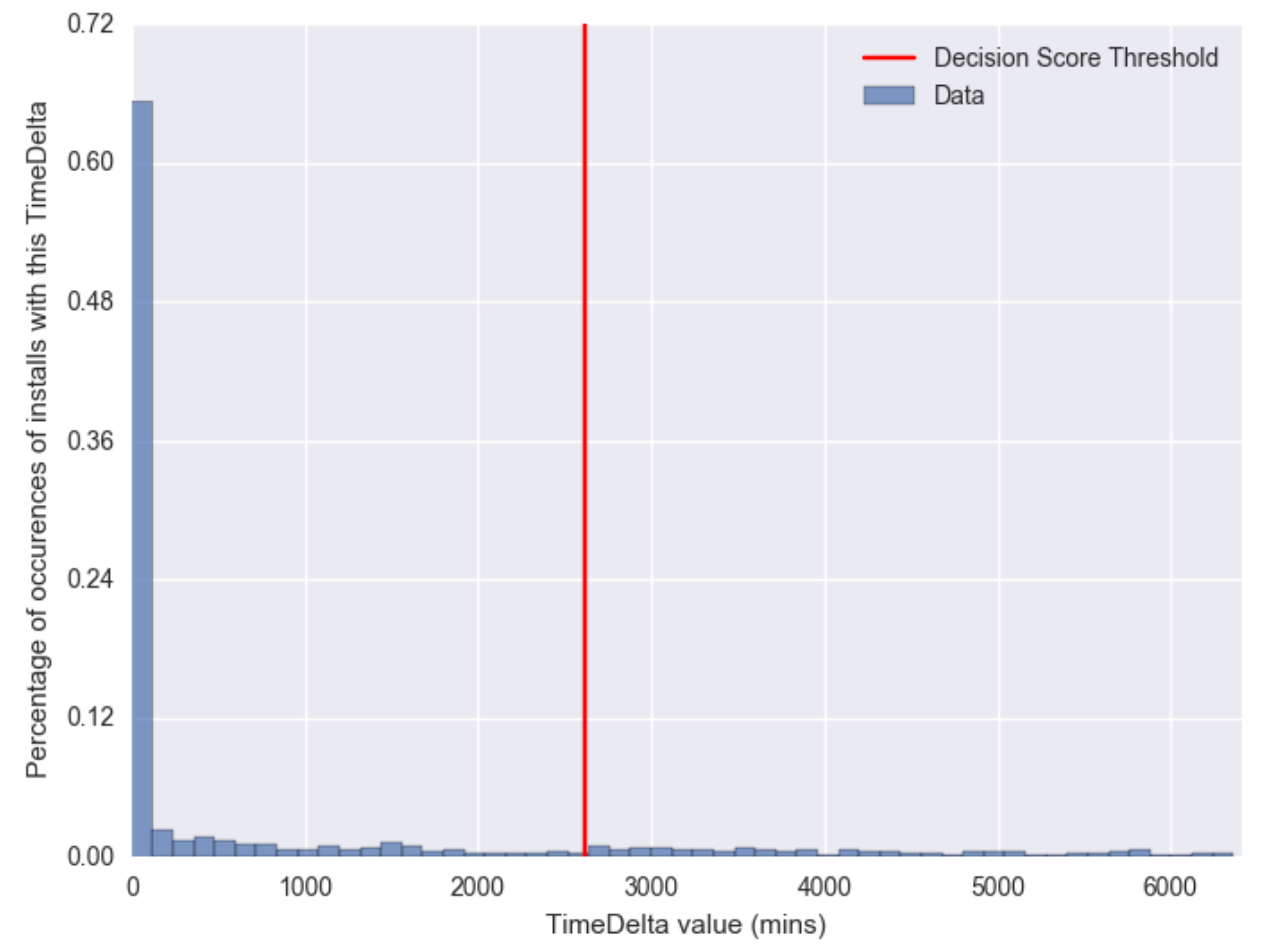
In this image bins are grouped every one hundred minutes. This sample shows all values extremely wrapped around minimum values, where the 95th percentile value is slightly over a day and a half.

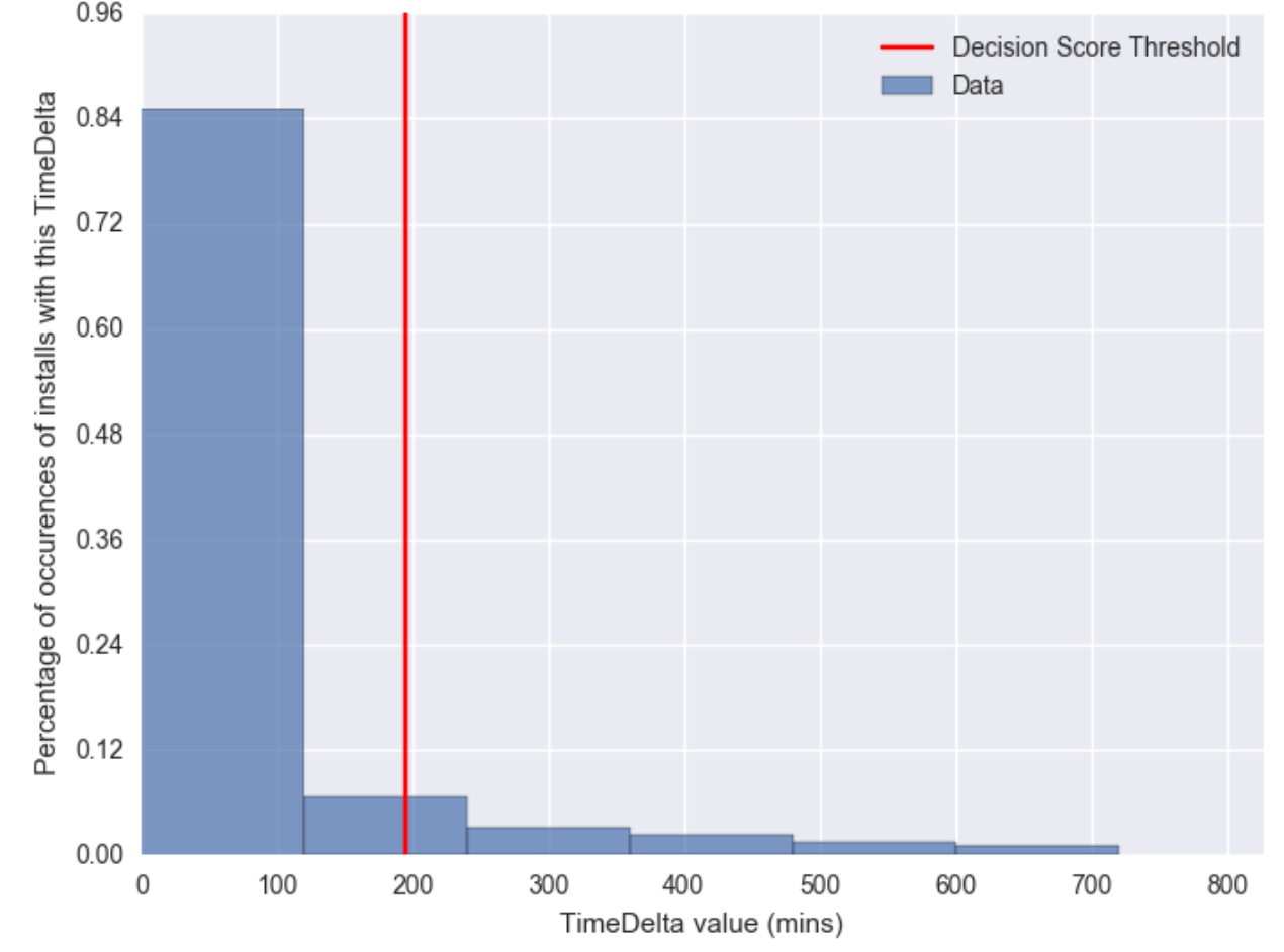
For this case we see a similar behavior but we find the decay to be much faster. The tail is much shorter than before and the threshold is set slightly over three hours. This is significantly different to the previous case.

Finally, to build an install threshold for today’s date, we take a timespan of data and record all of the thresholds calculated from those cases which were not regarded as coming from fraudulent behavior. From this data, we calculate the median threshold for each app and this value will be our cut. The median statistic has the advantage of being robust to outliers and this is important for cases where fraudulent behavior has slipped through as “normal”.

Conclusion

The methods here exposed are a first iteration for fraud detection and classification for Click Spamming. Note here that we rely on the assumption that for all apps there are periods free of fraudulent behavior. These periods are then used to calculate our final threshold which is robust to data that is contaminated. We are confident on this assumption since we have seen that fraudulent behavior from publishers will only last, at most, for a few days. Thus using at least one week of data is enough to identify cases of fraudulent behavior.

We find that this algorithm is strong and flexible to account for differences among applications, where there are significant time differences between TimeDeltas. The evaluation measures this difference by automatically fitting the best distributions for different contexts, which creates a robust and thorough fraud detection system.

References