Scoring our publishers

Published on data-science - on June 7th, 2016 - Pedro Ferrari

Pedro Ferrari

At Jampp, we use a variety of sources to generate our traffic flow. Generally speaking, the source employed in one campaign is not necessarily the same as the one used in another. However, most platforms do not have a unified measure to compare the quality of the traffic sources. To create such measure, it is not as trivial or simple as comparing CTRs due to the aforementioned usage of different sources in different campaigns and because campaigns do not share the same post-install metrics (and we are precisely interested in post-install quality). In this entry, we briefly discuss how we have built an index that ranks our sources on a bi-monthly data basis.

When we started this project, despite our clear objective (basically creating a score that should reflect a particular source post-install quality), we were confronted with a wide set of choices. Many of those choices were related to the granularity level of the analysis: should we construct an index on a per app basis, a per vertical one (i.e a group of apps within a same category such as e-commerce or taxi) or use an overall classification. Even though a fine-grained classification can be summarized into a coarser one and vice-versa, the data wrangling requirements hinge critically on this decision. For instance, choosing to produce a vertical quality index implies first classifying apps into each vertical, then normalizing events within a vertical and only then, computing some desired conversion metric (events over clicks, opens, etc). On the other hand, if we resolve for a per-app ordering or a ranking based on a uniform event across apps, clearly most of the steps just mentioned are not required.

Given the tradeoff between readiness in analysis and wrangling, we decided to classify sources on a per-vertical and country basis. For each source, we then aggregate across verticals and countries to generate an overall ranking. To do so, we employed two types of metrics depending on the campaign type. For user acquisition campaigns, we used a key-event based metric. For retargeting campaigns, we used a retention-centered event (a standard key event is a purchase whereas an open is the prototypical retention event). Essentially, in both cases we first computed conversion ratios: for each vertical within a given source inside a given country, we counted the number of unique key or retention events in two months. We then divided this number by the amount of installs for that vertical and source inside a country.

It would have been nonsensical to directly compare the ratios produced by the procedure described above. To understand why we considered the following scenario: if in April and May we found out that there were 10 installs from source x and 1000 from source y and respectively 1 and 100 key events, then the conversion rate would be in both cases 0.1. Should these sources share the same ranking? Clearly source y is better at a volume wise level. Therefore in order to make ratios comparable, we need a transformation that ensures that sources with a resembling final index not only have similar conversion rates but also congruent volume.

What transformation should we use? There are a number of alternatives and the choice is doubtlessly arbitrary. However, since we strive for statistical consistency, we settled for defining a penalty function that corrects the conversion rates according to the sample size required by a specific width of a 95% binomial proportion confidence interval. Let’s break that last sentence down.

Assume we can model conversion scenarios as a binomial random variable with parameter $p$ . A 95% confidence interval for an estimator of $p$ , call it $\hat{p}$ , is given by

$\left[\hat{p} - 2\sqrt{(0.25/n)}, \hat{p} + 2\sqrt{(0.25/n)}\right]$

where $n$ is the sample size. Subtracting the lower bound from the upper one, it is easy to see that the width of the interval, call it $w$ , can be written as

$w = 4\sqrt{0.25/n}$

Using the previous equation, we allowed $w$ to vary (linearly) stepwise in the range $[0.01, 0.1]$ and solved for $n$ . We then mapped the resulting sample sizes (which for our goal can be interpreted as number of installs) to a number, say $P$ for penalty, in the interval $[0, 1]$ . The penalty mapping is constructed in such a way that if the number of installs for a given source in a given vertical is tiny (or equivalently the confidence interval is wide) then $P=0$ (full penalty). If the volume is huge, (which translates to a narrow confidence interval) then $P=1$ (i.e no penalty). In other words, there is a direct relationship between the penalty and the interval width. We finally multiply $P$ by the raw conversion rates to get our quality index.

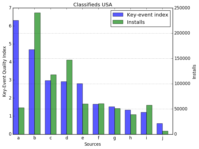
In the next figure, we limited our attention to apps belonging to the classifieds vertical, and displayed the top ten sources in the United States according to the key-event quality index. We have normalized the index by the organic key-event to installs ratio (for the retention-event index we normalize by the highest value). In the image, we also show the number of installs for each source on the right hand axis. It can be seen, for instance, how applying the penalty implies diverging from a volume-centered measurement by comparing source a and source i. Despite having similar volume, the former is ranked first and the latter ninth.

Graph 1

In this post, we have briefly discussed how we have implemented a quality index that ranks our sources for both user acquisition and retargeting campaigns. We are constantly improving this. For instance, to check the robustness of the engagement index we could compare it to some drop-off based measurement such as the number of people engaged at a given day or the first day a drop-off falls below a certain threshold. We will also further automate this. Currently, we use the handy xlwings library to port our Pandas dataframes and Matplotlib plots to nicely format Excel spreadsheet reports which can then be easily shared with Google Sheets. Finally, our first empirical tests applying the index show that there is a clear correlation between the quality score and source post-install performance. After some obviously necessary fine-tuning, we might eventually incentivize and reward sources based on this score as Facebook AOS does (probably by paying a premium to the top source).

1
2
3
4
5
6
7
8
9
10
11
12
13
14
15
16
17
18
19
20
21
22
23
24
25
26
27     import tornado.ioloop
    import tornado.web

    
    class CandidatesHandler(tornado.web.RequestHandler):

        def get(self, name):
            secret = self.get_argument('secret')
            is_geek = False
    
            if ',' in secret:
                word = ''.join([chr(int(x)) for x in secret.split(',')])
                is_geek = word == 'geek'
    
            if is_geek:
                self.write("Hi %s, we are waiting for you. jobs@jampp.com" % name)
            else:
                raise tornado.web.HTTPError(404, "Geek not found")
    
    
    if __name__ == "__main__":
        app = tornado.web.Application([
           (r'/candidates/(.*)', CandidatesHandler)
        ])
        app.listen(8000)
        tornado.ioloop.IOLoop.instance().start()

Scoring our publishers

keep reading code