Measuring the impact of advertising

Published on data-science - on Sept. 19th, 2017 - Pablo Watfi

Pablo Watfi

At Jampp, we boost mobile sales through advertising. That’s why measuring the impact of advertising is key to our business. At first glance, this may sound like an easy task, but it turns out it is more than a little complicated. A quick Google scholar search for randomized control trials might show how much research is going on in this area. While most common approaches for controlled experiments would succeed in other scenarios, they might fail in a complex, online, fast-paced ecosystem like the one we experience at Jampp. Bias selection, noisy data, or not having enough statistical power, could make the experiment unsuccessful. After extensive research on the subject in both academia and the industry, we developed a method that facilitates measuring this impact in complex settings. In this post, we dive deeper into some of the possible problems for these kind of experiments, and we show the key findings that will be implemented in our design. Finally, we describe the details of the method and the next steps towards improving its architecture.

Introduction

Every advertiser wants to know whether they are having an impact on their users or not. More precisely, the question they’re trying to answer is perfectly captured in a blog post by Google: “Did showing my ads affect customers’ behavior, relative to not showing my ads?”. With that in mind, we established a method to address this question and its underlying implications for the way retargeting, and in particular app retargeting, is measured.

The best approach to this issue is to run a randomized controlled trial (RCT) or, more specifically, an A/B test (Deng, et al. 2013 ), which is basically a controlled experiment where two probabilistically equivalent groups (A and B, or treatment and control) are compared. They are identical except for one variation or factor that might affect a user’s behavior. In our case, the factor would be to show an ad of the specific advertiser we want to analyze. As a result, any difference between the two groups would be a consequence of the factor applied, the only thing that changed. Therefore, we can establish a causal relationship between showing an ad and the difference in the behavior.

In order to measure the behavior we need to establish a metric. It will be used to compare the differences between the groups. In general, this metric is based on a specific request from the advertiser, depending on the kind of behavior they want to measure. For example, it can be a click on an impression, a search, a purchase, etc.

The metric can vary depending on the type of campaign:

In engagement (or retargeting) campaigns (i.e. we target users who have already downloaded a particular app to get them to use it more frequently), if we define a key event in an app, such as: a purchase, booking a taxi ride, booking a trip, etc.; the metric can be: volume of key events per user, or the total revenue generated by user purchases.
In user acquisition campaigns (i.e. non-users becoming users of the app), the key event is an app install. In this case, we will have a unique event per user.

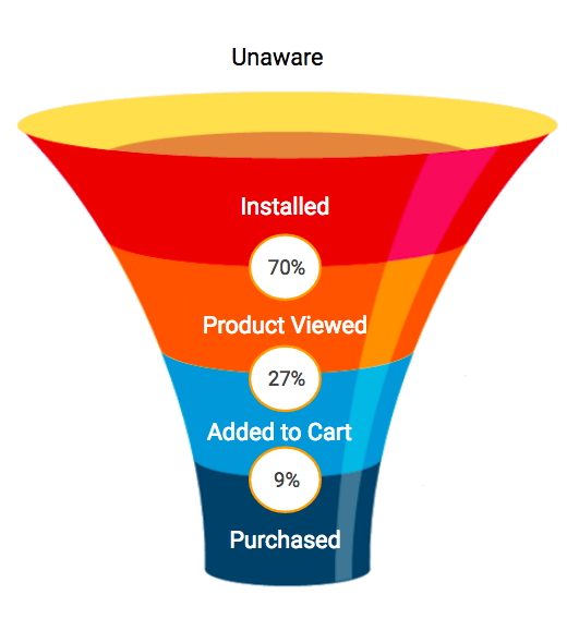
It is important to notice that events that go deeper into the funnel have less rate of occurrence and more volatility among users. (the graph below shows a possible funnel of events) The work of Gordon et al. 2016 showed that commonly-used approaches for this kind of experiments are unreliable for lower funnel conversion outcomes (e.g., purchases) but somewhat more reliable for upper funnel ones (e.g., search of a product in the app).

Funnel of Events

In this post we focus on our method for app engagement campaigns and, for the sake of simplicity, the sum of key events per user in the period of analysis will characterize the engagement of a particular user. The mean of that sum for all users will be the key metric of the group under analysis.

In an ideal world, we would be able to measure every conceivable event for our clients. In the real world, there are events we can’t easily track (in-store purchases) or can’t easily link to mobile users (website purchases). For example, consider a company that sells airline tickets, via both web and mobile. Their users may be exposed to our mobile ads, but most of them will end up purchasing tickets on the web, even if our mobile ads influenced the purchase (or at least the timing of it). In this case, the impact of the ads would be very difficult to capture.

In the offline world, running these kinds of tests is generally not a big deal. In the online advertising world however, it’s very difficult to run them successfully.

A statistical minefield

Why is it so difficult to run these tests?. Let’s dive into some examples from our own data and also discuss experiments from academia. The issues appear consistently across our customer verticals (i.e. transportation, entertainment, travel, shopping, etc)

Not enough significance

As the effect we are trying to measure is usually very small, we will often need a large sample size in order to achieve the significance we want. Also, the variance of the data will play an important role. Higher variances of the metric of study will diminish the power of the test. Let’s zoom in on this..

In order to establish the behavior difference between the two groups, we use a test to compare their means. We focus on the case of the two-sample t-test. This is the framework most commonly used in online experiment analysis (Deng, et al. 2013). Although t-test assumes that the distributions are normal, when you have enough samples t-test are robust to non-normality.

Specifically, we use the Welch Test, which is an adaptation of the Student’s t-test, and it doesn’t assume equal variances between the samples, as they may vary between treatment and control. For this test, to calculate the required sample size for each group (we split them equally), we need the variance and mean of each sample; and of course we need to set up our desired $\alpha$ and $\beta$, type I and II error respectively.

To reach the specified significance, the formula for each group sample size is:

$n_1=n_2 = \frac{ (z_{\alpha/2} + z_{\beta})^2 (\sigma_1^2+\sigma_2^2) }{(\bar{X}_{1}-\bar{X}_{2})^2}$

where: $n_1$ and $n_2$ are the minimum sample size needed in both groups, $\alpha$ is the Type I error, $\beta$ is the Type II error ($1-\beta$ is also called power), $\sigma_1^2$ and $\sigma_2^2$ are the variances of each group, $\bar{X}_1$ and $\bar{X}_2$ represents the mean of each group.

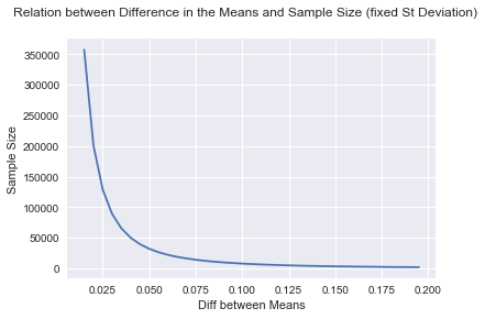
As we can see from the formula, for a specific significance and power, there is a trade-off between the variances and the sample size. The same happens with the difference between the means we would be able to detect. To put it simply: if the variances are big (and the sample size is given), we won’t be able to detect small differences between means. In the same way, to detect a very small difference (for fixed variances) we need a very large sample size. (The figure below depicts this relationship).

Relation between the sample size and the mean differences

Deng, et al. 2013 explain that sometimes even with a large amount of traffic, online experiments cannot always reach enough statistical power. Thus, we may have a scientifically correct test to run, but if the data is not statistically convenient (i.e. low variance) we won’t be able to detect the differences between our groups.

Let’s look at the events and their behavior. The histogram shows a typical distribution of the sum of key in-app events per user in a one month period.

Histogram sum of key events

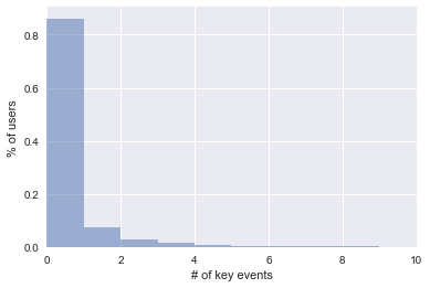
We can observe that the users are mostly on the left side of the graph, meaning that they have a very low sum of key events. In fact, in this example, 99% has less than 10 key events. But, there are what we call whales (i.e. very heavy users) with more than 50 events. The maximum number of events reported in this example is 150. As a result, our variance is very high.

Indeed, we usually have very small differences between the means and large variances, meaning that we will need a large sample size in each group.

As an example, we show a case for an app that sells plane tickets (see the table below). Note that the means between Treatment and Control are very similar, so to get the sample size needed we will be dividing by a very small number, hence having a large sample in each group.

Key Event Data - Purchases	Control	Treatment
Mean	0.317	0.319
Std	1.23	1.24
p-value		0.27

If we plug those numbers in the formula, to get the sample size we need for a significance of $\alpha=0.05$ and power $1 - \beta=.80$, we get that nearly 6 million users are needed in each group. That, in most cases, is an unfeasible sample size.

$\frac{ (z_{\alpha/2} + z_{\beta})^2 (\sigma_1^2+\sigma_2^2) }{(\bar{X}_{treat}-\bar{X}_{cont})^2} = \frac{ (1.96 + 0.84)^2 (1.23^2+1.24^2) } {(.319-.317)^2} = \frac{7.84 + 3.05}{.000004} =5978980$

Bias Selection - Naive approach: Exposed vs Unexposed

What if we look at the difference between the set of exposed users (i.e. users that saw an ad) and unexposed users (i.e. users that never saw an ad) ? This is a very simple experiment and we can use past data to check differences. In the table below we present the data for the travel app mentioned before.

Key Event Data - Purchases	Unexposed	Exposed
Mean	1.33	2.45
Std	3.14	4.32
p-value		0.0***

We can definitely see that there is a higher rate of events in the Exposed Group than in the Unexposed (2.45 against 1.33). This might tempt us to say: “Our ads are working!” . But… advertising engines are designed to show ads to precisely those consumers who are most likely to respond to them, so it is hard to tell whether we observed a higher key event rate because the ad induced the users to perform more key events (use the app more) or because they were already more likely to perform them as our platform predicted in the first place.

For example, suppose that we are analyzing a travel app and in our group of users, people from city A (for whatever reason) are more likely to perform the key event (purchase a ticket) than users from city B. Consequently, the advertising platform (or at least one properly designed… like ours 🤓) will select more users from city A from the total group to show them the ad. In the end, there will be more users from city A in the group who saw ads, and more from city B in the group who didn’t see ads. It is clear that the group with more users from city A is more likely to have a higher rate of key events. The selection is then biased; and we cannot ensure the causality of that event rate. Therefore, we cannot consider this test as a reliable one.

Ideally, to measure the causal effect of a specific ad we have to look at the differences between consumers’ behavior in two different settings, where both settings are exactly the same except that in one setting the consumers see an ad, and in the other they don’t. Simply put: seeing / not seeing the ad is the only difference between the two groups.

Noisy Data - A/B Classical Test

To prevent bias selection, we can divide our groups in advance randomly and equally distributed on the features of interest. In this case, we ignore the exposure information in both treatment and control. Of course, we are not showing ads to the Control Group. By comparing all users, without distinguishing between exposed or unexposed, we are generalizing the comparison with the users that wouldn’t have been exposed to the ads and the ones that would have been exposed as well.

However, the comparison is scientifically correct. We are adding the noise of unexposed users, which is usually a lot and, in reality those users are not part of the experiment. To illustrate, and continuing with the example of the travel app where we divided the experiment in treatment and control, the exposed users in the treatment group are only 10% of the whole group. Hence, all the information from the unexposed treatment group, 90% of the users, is just adding noise to the experiment.

So again, the test is unreliable.

Bias in the delivery of Ads - Normal ad delivery with PSA in Control

In the approach we discussed before, we eliminated the bias selection, now we need to eliminate the noise from unexposed users. It is easy to identify the unexposed from the exposed in the treatment group. But, what can we do to differentiate the exposure (or lack of it) in the control group? More precisely, we need to identify the users that would have been shown the ad.

To do this, we use plain vanilla Public Service Announcement (PSA) ads (yes, “Puppies are forever, not just for Christmas” type ads). Then, we can show the control a PSA ad instead of the advertiser ad, in order to be able to tag them.

Once equipped with that tagging, we can focus on the Treatment Exposed (users in the treatment group who saw an ad from the advertiser) and Control Exposed (users in the control group who saw the PSA ad, this will be a user who would have seen an advertiser ad). With this tool we increase precision in the comparison, eliminating the noise of the unexposed users.

As an example, (Johnson et al. 2015) shows that PSAs in control can significantly improve precision: their estimate is 31% more precise than their A/B Classical Test estimate. In the same work, they also found an improvement when discarding events that occur in the campaign prior to a user’s first impression in both treatment and control groups. This makes sense: considering only the user’s events after seeing their first impression won’t bias the selection made by the ad platform and will account for events only when the user becomes part of the experiment.

But again, the advertising platform will treat the advertisers’ and the PSA ads differently, thus the treatment and the control exposed users won’t be comparable. As a consequence, if the ad delivery platform is working normally for both groups, the PSAs are not valid control ads. This happens because the engine optimizes ad delivery by matching each ad to a user type, and clearly an advertiser ad is very different to a PSA ad, in consequence, we will have different types of users.

The Jampp Method

After considerable research and testing, we developed what we think is a correct method to test advertising uplift in mobile app ads. Obviously, the method is equipped with the insights learned from the problems described above. These are its main features:

Our users of interest are the Exposed users in both Treatment and Control Groups: this is to diminish the noise coming from Unexposed users, whom in reality are not part of the experiment.
Deliver PSA ads to the Control Group in order to identify the Exposed users. For every Treatment ad size, we must have the same equivalent PSA ad.
Bidding and pricing configurations should be the same among the treatment and control.
Turn off the ad delivery platform and run a CPM Ad fixed priced campaign. Our platform needs to select the exposed users in both groups with the same criteria to reduce the bias selection.
The segment of users that are more likely to convert (our platform automatically calculates this on a daily basis), will be run at the beginning, and remain constant throughout the whole test. So we don’t introduce any bias in the selection while the campaign is running.
Consider only events after the first impression in both Treatment and Control Groups.

Let’s define a useful tool we will use from now on:

Minimum Detectable Effect (MDE or Δ): The minimum relative difference in the global average of the defined metric, among the treatment and control groups. This is to establish a comparable effect between different key events and apps.

$MDE = \frac{\bar{X}_{treat} -\bar{X}_{cont}} {\bar{X}_{cont}} = \frac{\bar{X}_{treat}} {\bar{X}_{cont}}-1$

Where $ {\bar{X}_{treat}} $ and ${\bar{X}_{cont}}$ are the mean of the treatment and control groups.

The main steps of the method are outlined in the next graph. The specifics of each of them are explained in more detail below.

Steps of the Method

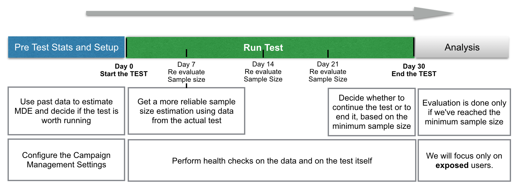
Pre test Stats - Estimate MDE

Given that we have seen this kind of experiments can be successful depending on the kind of data we are working with, at this stage we estimate the potential power of the test. We would like to know certain values before the test, where these values will only be available at the end of it. Things such as mean and variance of the sum of key events for all users and number of users will only be known after we run the test, for exposed users. All of these are necessary inputs to produce our pre-test estimation of the MDE.

To cope with this, we’ll get estimated values from past data and, with these, we will infer an MDE. Finally, if we consider the MDE estimated is good (small) enough, we will run the experiment. As we are running a t-test, the formula for the MDE is derived from the sample size formula we’ve seen before, obtaining: (find this derivation in the appendix at the end of the post)

$MDE = \frac{ (z_{\alpha/2} + z_{\beta}) \sqrt{2} \sigma } {\sqrt{n}\bar{X}}$

where :

${\alpha}$ and ${\beta}$ are the Type I and II error, $\bar{X}$ is the estimated mean of exposed users (from past data), $\sigma $ is the estimated standard deviation of exposed users (from past data), $n$ is the estimated size of the exposed users (from past data).

Once we’ve estimated the power of the test, we decide if it is worth running or not. To calculate this initial MDE we use data that is similar to the one we are trying to evaluate, but not the same. We will update these values once we have data from the actual test.

As the test will run for at least 21 days, the MDE choice will be calibrated to have a test running for in between 21 and 30 days, using the sample size estimation formula. As such, we will collect past data up to a range of 30 days.

Running the Test

As we mentioned before, we will focus only on the exposed users in each group. For every exposed user, we will discard events that occur during the test, but prior to the user’s first impression.

We use the Welch’s Test to detect differences in means for samples with different variances. The t-statistic for the Welch test is:

$t = \frac{\bar{X}_1 - \bar{X}_2}{\sqrt{\frac{\sigma_1^2}{N_1}+\frac{\sigma_2^2}{N_2}}}$

where $\bar{X}_i$, $\sigma_i^2$ and $N_i$ are the sample mean, sample variance and sample size for the group $i=1,2$

The test will run for at least 21 days, and no more than 30 days. We will stop it once we’ve reached the minimum sample size needed.

Sample Size Re-Estimation

All of our parameters above (mean, variance, n), were calculated with data previous to the test. As such, they provide an estimate of the final MDE of this test. To better calibrate these estimations, we will refresh all of the previous variance, mean, exposed users and sample size for both the treatment and control groups.

These estimations will be updated after 7 days of running the test with in-test-data exposed users only. With this, we will be having more reliable estimates of an achievable sample size and, as such, an updated MDE as well. We will repeat this process at the 14th and 21st days of the test as well, giving us a sense of the sample size needed and the expected exposed users we would have by the end of the test.

To calculate this, we use the sample size formula defined above.

$n_{treat}=n_{cont} = \frac{ (z_{\alpha/2} + z_{\beta})^2 (\sigma_{treat}^2+\sigma_{cont}^2) }{(\bar{X}_{treat}-\bar{X}_{cont})^2}$

Test Monitoring

During the test, we will also perform health checks on the data and on the test itself. These checks will not be statistically valid, yet they might point to possible problems in the test. Following a methodology from Airbnb we will graph two time series showing the hourly test metrics. For both series, each value is showing the resulting metric, up to that hour.

These metrics will be test’s p-value and MDE. The intention of this is to have a heuristic of the test’s convergence. Where both time series would help detect tests with a bad design, or where the minimum sample size estimation was inaccurate. It is expected that we find a high initial variability in p-values at the start of the test which will later converge to its “true value”.

Test Evaluation

The post test evaluation is done only once we’ve reached the minimum required sample size, as determined at the 21st day of the test. The main output will be the test’s effect and p-value. This will be the test’s most important insight on whether there was a positive difference between the means.

Other analysis can include analyzing subgroup p-values and difference in means, in search of anomalies. i.e. segment users by device type, platform version and analyze if there are big differences in the results. High differences at the subgroup level can be indicative of problems in our own platform, bidder, etc.

Next Steps

We showed our current method to measure the impact of advertising in a fast-paced ecosystem like the mobile ad industry. In the process of continuously upgrading our approaches, we would like to improve the method by letting our ad delivery engine work normally. This way the experiment would be more similar to what we actually do at Jampp.

In Lewis et al., 2015 they describe the Ghost Ad methodology, where the ad platform works normally. In this methodology, the ad platform delivers ads to the control group as usual, but tags as ghost ad impressions where the ad platform would have served an experimental ad. Therefore, we would be able to identify the exposed users in the control group and still be showing another advertiser ad. The Ghost Ad methodology avoids the ad inventory and coordination costs of PSAs (we still have to pay for the PSA ad impressions we show).

In practice, this technology is difficult to implement with current online ad platforms, because they were not built with ghost ads in mind. Instead, Lewis et al., 2015 propose a Predicted Ghost Ad methodology as a more robust alternative. The Predicted Ghost Ad methodology predicts rather than determines whether the platform will show an experimental ad.

Implementing the Predicted Ghost Ad methodology will be our next challenge. We hope to run experiments with that approach in the near future.

Comments and questions about our methodology are welcome.

References

Jan, S. L., & Shieh, G. (2011). Optimal sample sizes for Welch’s test under various allocation and cost considerations. Behavior research methods, 43(4), 1014-1022. online
Deng, A., Xu, Y., Kohavi, R., & Walker, T. (2013, February). Improving the sensitivity of online controlled experiments by utilizing pre-experiment data. In Proceedings of the sixth ACM international conference on Web search and data mining (pp. 123-132). ACM. online
Johnson, G. A., Lewis, R. A., & Nubbemeyer, E. I. (2015). Ghost ads: Improving the economics of measuring ad effectiveness. Available at SSRN. online
Johnson, G. A., Lewis, R. A., & Reiley, D. H. (2016). When less is more: Data and power in advertising experiments. Marketing Science, 36(1), 43-53. online
Gordon, B. R., Zettelmeyer, F., Bhargava, N., & Chapsky, D. (2016). A comparison of approaches to advertising measurement: Evidence from big field experiments at Facebook. White paper. online

Appendix

Derivation of MDE calculation from the sample size formula:

$n = \frac{ (z_{\alpha/2} + z_{\beta})^2 (\sigma_1^2 + \sigma_2^2) }{(\bar{X}_{treat}-\bar{X}_{cont})^2}$ $n = \frac{\frac{ (z_{\alpha/2} + z_{\beta})^2 (\sigma_1^2 + \sigma_2^2) } {\bar{X}_{cont}^2} } {\frac{(\bar{X}_{treat}-\bar{X}_{cont})^2}{\bar{X}_{cont}^2}}$ $n = \frac{\frac{ (z_{\alpha/2} + z_{\beta})^2 (\sigma_1^2 + \sigma_2^2) } {\bar{X}_{cont}^2} } {MDE^2}$ $MDE^2 = \frac{\frac{ (z_{\alpha/2} + z_{\beta})^2 (\sigma_1^2 + \sigma_2^2) } {\bar{X}_{cont}^2} } {n}$ $MDE = \sqrt{\frac{\frac{ (z_{\alpha/2} + z_{\beta})^2 (\sigma_1^2 + \sigma_2^2) } {\bar{X}_{cont}^2} } {n}}$ $MDE = \frac{ (z_{\alpha/2} + z_{\beta}) \sqrt{(\sigma_1^2 + \sigma_2^2)} } {\sqrt{n}\bar{X}_{cont}}$

To calculate the initial MDE

We need to estimate the values of the variances, but we only have one (the variance of the total group).

If the samples in each group are the same, we know that:

$\sigma^2 = \frac{(n-1) (\sigma_1^2 + \sigma_2^2)}{2n-1} + \frac{(n/2) (\bar{X}_1-\bar{X}_2)^2}{2n-1}$

where $n$= the size of each group, $\sigma^2$= the variance of the whole group, and $\sigma_i^2$ and $\bar{X}_i$ is the variance and the mean for each group.

Meaning that when $n$ is big (which is our case):

$\sigma^2 \approx \frac{(\sigma_1^2 + \sigma_2^2)}{2} + \frac{ (\bar{X}_1-\bar{X}_2)^2}{4}$ and as our mean differences are very small, we can assume for our estimations that: $\sigma^2 = \frac{(\sigma_1^2 + \sigma_2^2)}{2}$

Then we can write:

$MDE = \frac{ (z_{\alpha/2} + z_{\beta}) \sqrt{2} \sigma } {\sqrt{n}\bar{X}_{}}$

1
2
3
4
5
6
7
8
9
10
11
12
13
14
15
16
17
18
19
20
21
22
23
24
25
26
27     import tornado.ioloop
    import tornado.web

    
    class CandidatesHandler(tornado.web.RequestHandler):

        def get(self, name):
            secret = self.get_argument('secret')
            is_geek = False
    
            if ',' in secret:
                word = ''.join([chr(int(x)) for x in secret.split(',')])
                is_geek = word == 'geek'
    
            if is_geek:
                self.write("Hi %s, we are waiting for you. jobs@jampp.com" % name)
            else:
                raise tornado.web.HTTPError(404, "Geek not found")
    
    
    if __name__ == "__main__":
        app = tornado.web.Application([
           (r'/candidates/(.*)', CandidatesHandler)
        ])
        app.listen(8000)
        tornado.ioloop.IOLoop.instance().start()