The importance of serving the right amount of ads

Published on data-science - on Jan. 12th, 2018 - Juan Mateo de Monasterio

Jampp¹ helps customers boost their mobile sales with performance marketing. One of the most challenging problems of the industry is quantifying the impact an ad has on users. Understanding when a user has seen “enough” ads and reconciling click acquisition with the interests of performance advertisers have historically been difficult problems to tackle. We know that, sometimes, serving more impressions to users will result in CPA increase, since we can not influence their behavior any more. The key question is: how many ads are enough?

Introduction

Performance advertising is relevant to advertisers that want to have a quantifiable measure of their ROI. This means that the investment in advertising has to reach measurable goals such as increased number of in-app activity or app downloads. Then, the payment is directly measured by the value brought by the events caused by ads.

RTB ad platforms all enforce value prediction at the user and creative level. These typically take into consideration information history from the auction itself, or from the advertiser’s campaigns, but little effort is put on the user’s history of impressions.

Today, advertisers spend millions in marketing budget among different partners. They have to determine who takes the credit for making the user convert, in other words, which partner is the action attributed to.

Current attribution methods rely on what is known as the last-touch of a user. Where “touch” refers to either impressions (ad views) or clicks generated by that user, prior to the conversion. By far, the most widely used method is last-click. Still, from our analysis we have seen that there is a great amount of value driven by impressions that goes unaccredited.

We understand that, all other things equal, a user which has repeatedly seen an ad for a short period of time should not be treated the same as one which has seen it with less frequency. Yet quantifying the effects of advertising on both these types of users is hard.

At the same time, how much value do impressions drive? It is clear that they play a key role in advertisers’ efforts to reach/engage users, but the current industry pricing models compensate deeper funnel interactions, i.e. clicks or events. Yet impressions are relevant.

Another element to consider when assessing impression value is what the industry refers to as “frequency capping”. From our research, there are not many articles published on this subject: a user’s functional relationship of the number of impressions a user is served and the likelihood of performing a desirable action, be it an install or an in-app-event.

We make an initial approximation on establishing a limit to the amount of advertising messages shown to a unique user, expanding on this topic’s technicalities, problems, perspectives and first methods to analyze the data.

Our simulation stems from the idea that we have to dynamically limit the number of ads that a user will see during a given campaign, to minimize excess spending and improve Cost Per Action (CPA). Based on some assumptions, we detail a method to calculate the optimal number of impressions that should be served to a user for a given campaign.

The RTB ecosystem

In the most simple RTB ad space, there exists a marketplace consisting of three groups of players: advertisers, publishers and exchanges. App marketers demand advertising spaces in exchange for money and the publishers supply those spaces. Here, the exchange acts as an intermediary between these two groups and directs the flow of users in one direction: publishers $\rightarrow$ advertisers. Also, it oversees the money flow in the opposite direction.

Virtually all RTB exchanges offer ads by means of auctions which operate under the second price model i.e. the winner will not pay their actual bid price, but the second highest bid price.

Keep in mind that in the RTB space, performance advertisers are paying for impressions but their bottom line is to get users to spend more time or money in their apps. Showing ads is a means to an end, and it’s not without its risks. Advertisers come to us to minimize the risks and uncertainties of the ad space buying process. Clients would spend in advertising only conditioned on user actions and we, in turn, have to optimize the advertising spend to reach those objectives. When bidding, we optimize our pricing strategies to effectively minimize the risk using machine learning techniques in a scalable way. We can optimize these decisions at a rate of millions of times per second for a number of geos, clients, platforms, etc.

Our bidder then bridges between the CPA and CPM pricing models. This must be done in the most effective way for our advertisers. Part of this task means having an optimal frequency-cap for impressions.

Analysis

To start, we must analyze our current last-touch attribution model. By touch we might either refer to impressions or clicks. In both systems in which the advertiser will retribute the publisher who was the last to show an ad to the user, prior to their conversion.

The retribution is always conditional to the message being delivered within a predefined attribution window. These windows are set as a method to incorporate causality in the model. It is safe to say that a click that occurred one year prior to a conversion has no relationship to this event.

For clicks, this window is typically set between seven to thirty days, whilst for impressions, it is commonly set to twenty four hours. While the industry believes there is a significant causality relationship between seeing an ad and actually going forward and, for example, purchasing a shirt, the purchase is seen nearer to a click. Here, it is assumed that the user’s intent is stronger by their interaction with the ad (click), rather than only viewing the ad.

The ad life-cycle for a typical user might look something like this:

User life-cycle in advertising

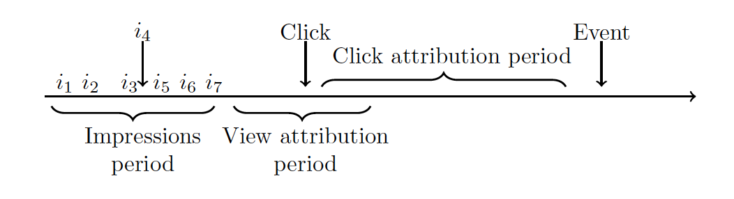
We can see that there are two possible attribution periods, caused by the different message types. These can overlap in time and they do not cancel each other.

The figure above is an example of a scenario where the user has only one conversion in his timeline. But conversions can happen a number of times over a given period. Users need not convert only once, and every time this happens there are systems checking the attribution of that conversion, to past impressions or clicks.

Note that this is just one of many possible user attributions. We could actually have more impressions after the click, or no click at all. A user can be for example buying goods, without actually clicking on ads.

Assumptions

From our messages, we search click, impression and conversion logs. Here we will be assuming that these logs are i.i.d random variables, for any given instance $c \in C$ (during a time period $T$).

We also make other key assumptions about our data’s structure. First, we say that a click is inextricably caused by its impression. There are no other factors affecting a click and this causality can not be shared among impressions. There is only one impression joined to that click. This affects our analysis when simulating different frequency cap levels. For example we will have that a frequency cap of eight, will cut all impressions of higher frequency number. With this, we will assume that a drop of an impression that is joined to a click will directly lead to a loss of that click. Yet this would not occur for events, where an impression loss (or click loss as well) would not necessarily incur in the event loss. Our assumptions structure attribution relationships among distinct message types in this way. The bottom line is that it is not the same to say we lost an impression for that click, than an impression for a conversion.

Finally, we will be setting attribution windows to the values most commonly used by our clients which are twenty four hours for last-impressions and thirty days for last-clicks.

Data Preparation

Consider a time window $T$ over which to analyze our data, fifteen days or one month, as a way of accounting for stationarity in the data.

Let $A$ be the set of apps (or Advertisers) and, without loss of generality, consider $a$ to be a generic app. The same goes for the set of Campaigns $C$ of those advertisers. In this context we can have multiple $c$ for each $a$, but each $c$ is assigned to one and only one $a$.

The set of users, clicks, events and impressions will be noted by $U$, $Cl$, $E$, $I$, respectively. All of these occur inside the window² defined by $T$. Our data will be made of impressions and clicks that happen inside an attribution window, relative to our event of interest.

For impressions, we will calculate their frequency number. This is determined as the number of impressions a user receives per day. We will also refer to this as the impression number of that message. This is independent of the message being attributed or not.

In short, given a time period $T$ and a campaign $c$ we will want to have, for each $e$, the corresponding clicks ($cl$) and impressions ($i$) that occurred previous to $e$, under a user $u$. We will also check if the clicks and impressions comply with their attribution window, for that message type.

The above implies that for a certain user $u$ and a conversion $e$, we may have multiple associated clicks and impressions to that conversion.

Counterfactual Simulation

Here, we will consider only campaigns which had no actual frequency capping set during $T$. This is because we implement an offline counterfactual model where, for each $c$, we gather all messages as explained before, and hypothesize what would’ve happened had we frequency capped the campaign.

Consider $f \in F$ a frequency level threshold from the set $F = [1,\cdots,100] \cap \mathbb{N} $. With this, we can calculate a cumulative impression analysis. The idea is to look at the tradeoff when we simulate different frequency caps in the data, and output the resulting change in metrics. Naturally, all simulated capping scenarios would affect the volumes of clicks, impressions and conversions, and the spend of impressions.

Let us define some simple functions that formalize these notions. First, we need to know what is the resulting volume of impressions after the cap, by analyzing the data:

$Imp : F \rightarrow \mathbb{N} \\ f \rightarrow n$

The same goes for the remaining conversions volume after capping:

$Conv : F \rightarrow \mathbb{N} \\ f \rightarrow n$

As we’ve said before, a simulated capping implies losing clicks. We thus have a functional, unknown, transformation $h(\cdot)$ between impression and click levels that affect the final click volume:

$Cl : F \rightarrow \mathbb{N} \\ f \rightarrow h(Imp(f))$

These relationships were created from the data, yet we could not explicitly give closed-form formulas for them. From our explorations, different campaign instances showed different relations. In other words, we can fit the data for a single instance, a specific campaign and time period, yet these functions will change for other instances in a way which does not allow their generalization. So we worked each instance separately.

As a second step, we needed to define business metrics that are relevant for our customers. Different frequency cappings would produce different levels of them, because of how the relationships $Imp$, $Conv$ and $Cl$ vary along cap levels.

Being a performance marketing platform, we prioritized CPA (cost-per-action) optimization of our clients. At the same time, and given the industry’s last-click attribution system, our revenue stream is click dependent. We used click volume as a second relevant metric. In this way, we obtain two metrics defined as functions of the previous relationships.

Calculating CPA is very simple in terms of the average CPC (cost-per-click) for that campaign. It is easy to see that it is established as a functional relationship between $Cl$ and $Conv$.

$Cpa : F \rightarrow \mathbb{N} \\ f \rightarrow g(Cl(f),Conv(f))$

where $g$ is the functional relationship between both. Note that this metric is advertiser-specific.

We show here two examples of these relationships, for a specific campaign. The $Cpa$ and $Cl$ levels shown are evaluated at different frequency cap levels (x-axis). Note that the figures are given in terms of the percentage change, when compared to the baseline $Cpa$ and $Cl$ levels which exist when no frequency cap is enforced.

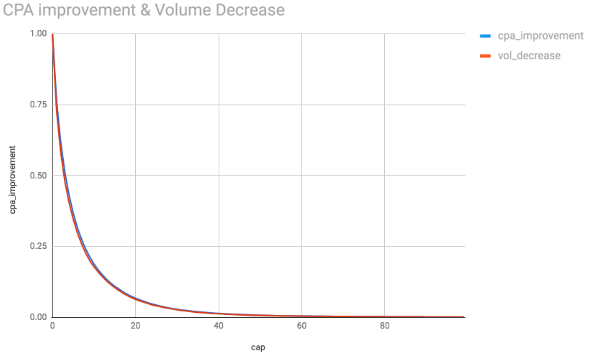
Comparison of both CPA and volume decreasing tradeoff series.

The tradeoff is very clear, at the minimum cap level and with one impression only we would have a huge optimization in CPA. The figures start at frequency cap level one, and by the looks of it we might think that this is the optimal CPA. Yet understand that this value is showing a singularity from the data. Such an extreme cap would imply barely any clicks for the advertiser and, in turn, barely any conversions volume.

We repeat the series above with another campaign, this is shown in the figure below.

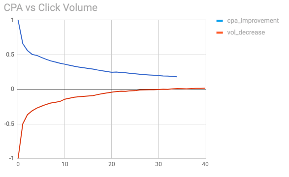
Side comparison of both CPA and volume series monotonous tradeoff for a different campaign.

Once again we see how the CPA is at maximum levels when the caps are at their minimum. Note how in this case there is a different functional relationship between the CPA and the cap level, in comparison to the previous figure. The same can be said for the volume decrease.

The question now remains: where do we set the optimal frequency cap, given these two metrics? This is a broad question which is more dependant on how the company values them. For our case, we decided to value both equally. We think this is both advantageous for us and our clients.

Given this multi-objective optimization setting, we scalarized the values in a single functional form. Valuing both equally means setting the same weights for both. Thus we find the optimal frequency cap level $f \in F$ by choosing:

$\mathrm{argmax}_{f \in F} Cpa(f) + Cl(f)$

as our optimal cap level.

Again, this valuation is something that suits our way of understanding the business. Different valuations create different optimization forms. We tried other ways, such as Pareto optimal relations, or other $\epsilon$-constrained methods. You can find more cool stuff about this topic on Wikipedia³.

The previous optimization yielded results which were more than satisfying. In general, we found that the optimal number of daily frequency caps per user was in between five to twenty impressions. This makes sense if we think that, when we want to get an advertising message across to a large group of people, we won’t get them immediately to convert. However, in general there is an amount of impressions which is just enough.

Final Remarks

Currently, we are simulating live campaigns with this method in order to model the would-be optimal frequency caps for them. Fulfilling these caps is important to manage a relevant amount of spend on the users and to efficiently provide quality to our clients. We think that intelligently buying media is most effective for our clients’ CPA.

We are also researching into other statistically valid methods on optimal frequency capping for performance where we play with other possible attribution models involving time decay patterns from the message to the conversion. We know that user behaviour can be caused by a variety of factors which, if recognized, would greatly improve our ad performance.

It is important for marketers to recognize the value in impressions and how they should be considered as part of the general view of how advertisements affect user conversions. At the same time, we understand there is excess spend in high-served users and this should be quantified. Frequency caps is a natural way of optimizing this situation where different methods, as shown above, can help to determine the optimal capping values. Iterating reports over these optimal cap values is detrimental to establishing intelligent campaign performance.

References

http://jampp.com/ ↩
We could possibly have events attributed to clicks occurring in the past. ↩
https://en.wikipedia.org/wiki/Multi-objective_optimization#Scalarizing ↩

1
2
3
4
5
6
7
8
9
10
11
12
13
14
15
16
17
18
19
20
21
22
23
24
25
26
27     import tornado.ioloop
    import tornado.web

    
    class CandidatesHandler(tornado.web.RequestHandler):

        def get(self, name):
            secret = self.get_argument('secret')
            is_geek = False
    
            if ',' in secret:
                word = ''.join([chr(int(x)) for x in secret.split(',')])
                is_geek = word == 'geek'
    
            if is_geek:
                self.write("Hi %s, we are waiting for you. jobs@jampp.com" % name)
            else:
                raise tornado.web.HTTPError(404, "Geek not found")
    
    
    if __name__ == "__main__":
        app = tornado.web.Application([
           (r'/candidates/(.*)', CandidatesHandler)
        ])
        app.listen(8000)
        tornado.ioloop.IOLoop.instance().start()